 |
 |
|||
|
In the following descriptions of test problems the notation will be used: n - dimension, The considered test problems are:
n=2, X=[-2,2]n f(x) = 100(x2-x12)2+(1-x1)2 f* = 0, X* = (1,1) , nloc = 1 n=2, X=([-1.5,4],[-3,4])
f* = -1.9133, X* = (-0.54719,-1.54719) , nloc = 1
Box and Betts exponential quadratic sum n=3, X=([0.9,1.2],[9,11.2],[0.9,1.2])
f* = 0, X* = (1,10,1) , nloc = 1 n=10, X=[2.001,9.999]n
Generalized Rosenbrock function n=30, X=[-n,n]n
f* = 0, n=2, X=[-2,2]n f* = 3, X* = (0,-1) , nloc = 4 n=4, X=[0,10]n
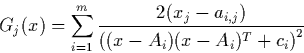
for m=7: f* = -10.4029, X* = (4.00057,4.00069,3.99949,3.99961 ) , nloc = 7 for m=10: f* = -10.5364, X* = (4.00075,4.00059,3.99966,3.99951 ) , nloc = 10 n=4, 5, 6, 7 for n=4: X=[-10,10]n for n=5,6,7: X=[-5,5]n
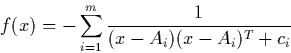
for n=4: f* = -21.502356, X* = (1,1,1,-9.752356 ) , nloc = 71000 n=10, X=[-500,700]n
f* = 0, n=2, X=[-5,5]n
f* = -1.03163, n=2, X=[-10,10]n
f* = 0
n=2, X=[-10,10]n
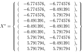
nloc = 400
n=2, X=[-10,10]n
f* = -176.541793
n=17, U=([0,4],[-4,4]n-1) x1 = y1 = y2 = 0, x2 = u1, xi = u2(i-2), yi = u2(i-2)+1
This problem was supplied by PhD student Per R. Andersen at IMM, DTU. It is a parameter estimation problem within a growth model of the human mandible (the lower jar). The data of the problem are the coordinates of 271 points of equivalent morphology from 3 mandibles of the same patient in the age of 9 months, 21 month and 7 years. The goal of the problem is to position three mandibles in the space so that the sum of distances of points from the middle mandible to the lines connecting points from the first and third mandibles would be minimal. The middle mandible is fixed and every of both others has 6 degrees of freedom: 3 angles of rotation and 3 directions of translation. n=12, The data are available here. |
|||
![\begin{displaymath} f(x) = \sum^{n-1}_{i=1}\CENTER[100(x_{i+1}-x_i^2)^2+(x_i-1)^2 \right] \end{displaymath}](img7.gif)
![\begin{displaymath} \begin{array} {cc} A = \CENTER[ \begin{array} {rrrr} 4 & 4 & 4... ...\ 0.3 \\ 0.7 \\ 0.5 \\ 0.5 \end{array} \right] \end{array} \end{displaymath}](img10.gif)