By Jeppe Revall Frisvad, 2019 (based on a paper on temporal glare [Ritschel et al. 2009] and a noise function [Frisvad and Wyvill 2007])
The iris muscles have the ability to control the size of the pupil. Exposition to a glare source will typically give rise to the pupillary hippus: an involuntary, periodic fluctuation of the pupil size. It is presumably caused by opposing actions of the iris muscles due to the vastly different lighting conditions of glare source and background when attempting to adjust the pupil [Murray et al. 2002]. The following curves describing the pupil diameter as a function of time for different glare source intensities have been measured by Fry [1991].
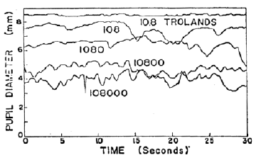
For a paper on temporal glare simulation [Ritschel et al. 2009], I found the following expression that mimics these dynamic: \[ h(t, p) = p + \textrm{noise}\left(\frac{t}{p}\right) \frac{p_{\max}}{p} \sqrt{1 - \frac{p}{p_{\max}}} \, , \] where $t$ is time (in seconds), $p$ is the mean pupil diameter (in mm) for a given glare source intensity, $p_{\max}$ is the maximum pupil size (we use $p_{\max} = 9$ mm), and noise($\cdot$) is a noise function. It remains to map glare source intensity to the mean pupil diameter $p$. We use the function proposed by Moon and Spencer [1944]: \[ p = p_{\max} - c\left(1 + \tanh\left[0.4(\ln(L_v\,\pi\cdot10^{-1}) + 0.5) \right] \right) , \] where $L_v$ is the field luminance measured in cd/$\textrm{m}^2$. Moon and Spencer [1944] used $p_{\max} = 7.9$ mm and $c = 3$. I slightly adjusted these parameters to better match the measurements by Fry [1991]. Thus, I use $p_{\max} = 9$ mm (as above) and $c = 2.5$. We may conjecture that Fry's measurements were conducted on a person with a large pupil. We can now implement a WebGL demonstrator that evaluates the function $h$ given above using the sparse convolution noise function by Frisvad and Wyvill [2007] with three octaves.
Inserting field luminance $L_v$ in the following box, you can control the simulated pupillary hippus displayed in the figure below. If you would like to mimic the curves by Fry [1991], you can divide by 92 to convert from Trolands to cd/$\textrm{m}^2$. It is not a perfect match. Some of the explanation is that Trolands measure retinal luminance and are defined by $T = L_v A_p$, where $A_p$ is the pupil area in $\textrm{mm}^2$, and this area changes with the field luminance. So, division by 92 is a rough approximation in our context.
$L_v = \:$ cd/$\textrm{m}^2$
The following figure is an attempt to reproduce Fry's figure using a Matlab implementation of the proposed formula.
