
[code] [lowres pdf]
| JEPPE REVALL FRISVAD | TOSHIYA HACHISUKA | and | THOMAS KIM KJELDSEN |
| Technical University of Denmark | Aarhus University | The Alexandra Institute |
Rendering translucent materials using Monte Carlo ray tracing is computationally expensive due to a large number of subsurface scattering events. Faster approaches are based on analytical models derived from diffusion theory. While such analytical models are efficient, they miss out on some translucency effects in the rendered result. We present an improved analytical model for subsurface scattering which captures translucency effects that are present in the reference solutions but remain absent with existing models. The key difference is that our model is based on ray source diffusion, rather than point source diffusion. A ray source corresponds better to the light that refracts through the surface of a translucent material. Using this ray source, we are able to take the direction of the incident light ray and the direction toward the point of emergence into account. We use a dipole construction similar to that of the standard dipole model, but we now have positive and negative ray sources with a mirrored pair of directions. Our model is as computationally efficient as existing models while it includes single scattering without relying on a separate Monte Carlo simulation, and the rendered images are significantly closer to the references. Unlike some previous work, our model is fully analytic and requires no precomputation.
|
Frisvad, J. R., Hachisuka, T., and Kjeldsen, T. K. Directional dipole model for subsurface scattering. ACM Transactions on Graphics 34(1), pp. 5:1-5:12, November 2014. Presented at SIGGRAPH 2015. [code] [lowres pdf] |
This WebGL example provides a comparison of two analytical dipole models for simulating subsurface scattering of light. We compare the standard dipole and our new directional dipole (see the figure below).
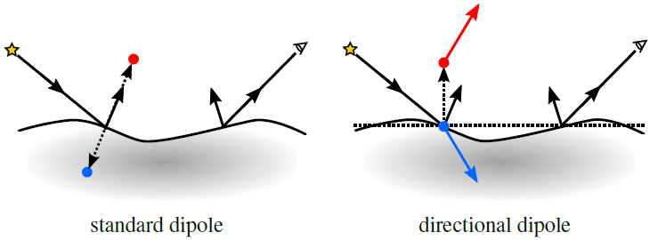 |
| Figure. A standard dipole model uses two point sources to handle boundary conditions. The points are displaced along the normal at the point of incidence. Our directional dipole model uses two directional sources that are displaced along the normal of a plane containing the points of incidence and emergence. |
To simulate subsurface scattering, we evaluate a bidirectional surface-scattering reflectance distribution function (BSSRDF) which depends on a rather large number of input parameters. The scattering material is described by a set of optical properties. In addition, the BSSRDF depends on the surface points of incidence and emergence, the surface normals in these points, and the directions of incidence and emergence of the light. We visualize the diffuse reflectance returned by the BSSRDF, which is a scalar. The optical properties and the intensity of the incident illumination (incident radiance) can be set in the following table.
| Incident radiance $L_i$: | |
| Scattering coefficient $\sigma_s$: | |
| Absorption coefficient $\sigma_a$: | |
| Asymmetry parameter $g$: | |
| Index of refraction $\eta$: | |
Diffuse reflectance due to approximate single scattering is added to the standard dipole model.
Mouse control: orbit - left button, zoom - middle button, pan - right button.
Keyboard options: larger angle of incidence - [+], smaller angle of incidence - [-], toggle colour mapping on/off - [m].
 | ||||
| $10^{-2}$ | $10^{-1}$ | $10^{0}$ | ||
The steps in the visualization pipeline of this example are as follows. To import data, we implement the BSSRDF in the shading language (GLSL) part of a WebGL program. The point of incidence and the normal at the point of incidence are set to constants. Optical properties, the eye point, and the direction of incidence are uploaded as uniform variables, while the point of emergence and the normal at this point are uploaded as vertex attributes and interpolated across the surface triangles using varying variables. In this way, we support sampling of the BSSRDF in an unstructered grid. To perform data filtering, we choose to draw a 4 by 4 by 4 cube and let the point of incidence be the centre of the top face with a fixed normal along the $y$-axis. The direction of incidence is in the $xy$-plane with an angle of incidence specified by user input. We also enable user modification of the incident radiance, so that the user can scale the visualization result. Since it can be hard to compare reflectance values if they are visualized as grey scale pixel intensities, we perform data mapping using a logarithmic function. We consider the result of this to be the hue and obtain a false-colour visualization using hsv to rgb colour mapping. Finally, the data rendering happens through the WebGL rasterization pipeline.